
Cold Storage Coupling for Portfolio Rebalancing in Crypto

The cryptocurrency space envisions a future which is open and decentralized. Although there are applications which are navigating towards this vision with trading, we are still a ways away from reliable solutions. Low liquidity, slow transaction times, and convoluted user experiences provide non-ideal situations. This isn’t to say these problems won’t be solved eventually, but at this moment, centralized platforms simply make sense for most investors. As a result, we need to be thinking about solutions to ensure the security of portfolios that are using centralized systems.
Unfortunately, there haven’t been good solutions up until this point. An epidemic of hacks has plagued the crypto space. Investors are faced with a conundrum. Whether they should manage their assets on an exchange, where they can maximize the potential of their portfolio or do they store assets offline and simply HODL. Neither answer is optimal, so making a decisive decision is still a struggle for most investors.
Today, struggle no more. There is a resolution to this difficult decision.
Rebalancing via Cold Storage Coupling
Cold storage coupling for rebalancing is the answer to this problem. When a portfolio is rebalanced, only the delta between the current and target allocation is traded. Since this is generally a small amount, only a limited percentage of the portfolio needs to be maintained online to completely rebalance. The rest of the assets can remain offline. These assets which are held in cold storage can then be considered as part of the portfolio during the calculations for rebalancing. Essentially, pretending the assets are online so all holdings are included during a rebalance. This provides a fair trade off between security, liquidity, and ease of use.
If you would like to learn more about rebalancing, you should start with the two following articles:
Portfolio Rebalancing for Cryptocurrency
Rebalance vs. HODL: A Technical Analysis
A Graphical Example
In the following section, we will define two different types of assets. There are assets which are online and there are those which are offline. Online assets are held on an exchange. These assets are liquid and can easily be traded between different assets. Offline assets are held in cold storage or any other 3rd party service. These assets are not liquid. These assets cannot be traded by the rebalancing tool.
The following figures will depict both online and offline assets. Online assets will be depicted as orange. Offline assets will be depicted as blue. The size of each bar graph is determined by the value of the asset. So, when an asset increases in price, the bar for that asset will get larger since the total value increased. When the price of an asset decreases, the bar will get smaller since the value of that asset has decreased. This means if two bars are the same size, they have equal value.
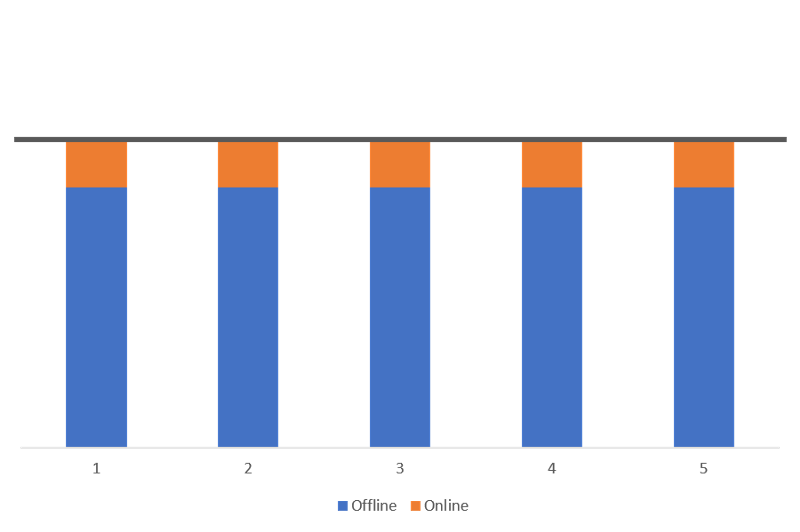
This figure shows a portfolio of 5 evenly distributed assets. The target allocation of each asset is therefore 20% of the portfolio.
In this example portfolio, we have selected 5 different assets. These assets are simply labeled 1 through 5 for simplicity. The bar graph indicates that each of the 5 assets is distributed evenly by value, so there must be a 20% allocation selected for each asset. Since we have even allocations, the target value for each allocation can simply be defined as the average. The dark line displayed on the graph is the target allocation line. This is the desired distribution for the portfolio across every asset.
The bar graphs indicate by the large blue segments that most of the value for each asset is held offline. These blue sections cannot be traded on the exchange, so to reach the target allocation line during a rebalance, the blue bar must always remain below the target allocation line.

This figure shows how the portfolio has deviated since the initial allocation. The target allocation for each asset is depicted by the dark line that intersects each bar graph.
In this example, after the portfolio is created, each allocation can deviate as the market value for each asset increases or decreases. This can be observed in the above image. When an asset increases in value, the blue and orange segments in the bar graph increase in size. In this case, asset 2 has outperformed the rest of the portfolio. This has pushed the blue segment of the bar for this asset closer to the target allocation.

This figure shows how the portfolio looks when it is rebalanced after a period of price movement. The target allocation for each asset is depicted by the dark line that intersects each bar graph.
Now, we will simulate a rebalance after the assets have been left to diverge for some time. The above image illustrates how the assets would be distributed after this rebalance. Although the allocations have deviated, there was enough of each asset liquid on the exchange to allow for a complete rebalance. However, it should be observed that the blue bar graph for asset 2 is getting close to the target allocation.
In this example, no intervention will be provided to prevent the value of the offline assets (blue bar graph section) from exceeding the target allocation line. In a real scenario, this is the time when an investor should take a portion of their number 2 asset from cold storage and move it online. This will increase the online holdings (size of the orange section of the bar graph) and ensure the offline assets (blue section of the bar graph) never exceed the target allocation line.
It can also be observed that asset number 1 has lost value. As it continues to decline in value, the asset will accumulate on the exchange. This provides an opportunity to remove some of asset number 1 from the exchange and send it to cold storage. This minimized the amount on the exchange and moves the blue bar graph section closer to the target allocation line.

This figure shows how the portfolio has deviated since the first rebalance. The target allocation for each asset is depicted by the dark line that intersects each bar graph.
Once the first rebalance is complete, each asset begins deviating once again. This results in each asset continuing to drift further from their initial distribution. The illustration demonstrates how the second asset has climbed past the target allocation line. This means the current value of the asset which is held offline is greater than its target allocation. To address this issue, some of the offline holdings of asset number 2 should be brought online so the next rebalance can execute properly.

This figure shows how the portfolio looks when it is rebalanced after a second period of price movement. The target allocation for each asset is depicted by the dark line that intersects each bar graph.
After a second rebalance, the blue section of the bar graph has climbed clear past the target allocation line. The image above demonstrates that after the rebalance is performed, the blue bar stays above the target allocation line. The reason is because this amount of the portfolio is not liquid. It is in cold storage which cannot be traded on an exchange. As a result, it not only can’t reach its target allocation, but no other asset can reach their target allocation. This is demonstrated by the white gaps that are seen between each orange bar graph segment and the target allocation line. To address this issue, some of the asset 2 which is located in cold storage must be brought online. The next rebalance would then allow the portfolio to reach the target allocations for each asset.
Tolerance Bands
Integrating cold storage for rebalancing can be furthered by incorporating tolerance bands. The example discussed above implemented a strategy where 85% of the initial value was held in cold storage. Since the deviation was great, this lead to incomplete rebalances when too much value was stored offline for an individual asset.
The solution to this problem is tolerance bands. The way this would work is by selecting a target percent that should be held in cold storage and the percent tolerance allowable for any given asset. An example of reasonable numbers would be a 90% cold storage target with a 5% tolerance. So, whenever an asset crosses above 95% of the target allocation being held offline, the investor should bring 5% of the target allocation in that asset online. Whenever the offline holdings cross 85% of the target allocation, 5% of the target allocation in that asset should be brought offline. The reason the value is calculated based on the target allocation and not the total value of the asset that is held in the portfolio is because rebalancing will attempt to reach the target allocation.
Cold Storage with Shrimpy
Shrimpy will continue to innovate on the way it allows users to secure their assets. While the current implementation is simple, optimizing the percent of assets that are maintained offline is an important aspect of the investment process. Whether you are an institutional investor or an individual, security matters to you.

This figure is a screenshot from a Shrimpy portfolio that uses this cold storage strategy.
Shrimpy implements these ideas through the “Cold Storage” feature on the dashboard side bar in the application. Looking at this example portfolio, we see the same pattern as the blue and orange bar graphs that were discussed above. In Shrimpy, these bar graphs are gray for “Cold Storage” assets and orange for assets on the exchange. As the orange section of the bar graph disappears, additional assets should be brought online to allow for proper liquidity. As the orange section of the bar gets larger, more assets can be brought offline. In the example above, we can see that approximately 80% of the assets are stored offline.

This figure demonstrates how “Cold Storage” balances are added to the Shrimpy application. Simply input the amount of each asset that is held in cold storage and it will instantly be included into your portfolio.
This image illustrates the simple way that you can add “Cold Storage” assets in Shrimpy. Simply select the asset that is held in cold storage and then specify the amount of that asset. For example, if you hold 1 DASH in a hardware wallet, simply select DASH and then enter 1 into the field and DASH will be added to your cold storage.
Additional Reading
The Whitepaper for Portfolio Rebalancing in Crypto
Crypto Users who Diversify Perform Better
The Crypto Portfolio Rebalancing Backtest Tool
10 Tips for Creating a Killer Cryptocurrency Portfolio
How to Avoid Scams with these 24 Cryptocurrency Red Flags
_ _ _
Don’t forget to check out the Shrimpy website, follow us on Twitter and Facebook for updates, and ask any questions to our amazing, active communities on Telegram & Discord.
Leave a comment to let us know your experiences with rebalancing!
The Shrimpy Team