
Backtesting the Best Crypto Strategies: Portfolio Rebalancing

Update 10/05/2022: New & Improved Shrimpy Backtest Tool Now Live
We are incredibly excited to announce that we have launched a completely overhauled backtest tab for the Shrimpy app! We heard feedback from many of you about wanting an improved experience for running backtests, and we are happy to say that this is now a reality.
The new backtest tab features a slick, responsive user interface, a massive improvement to the overall speed of running backtests, the ability to backtest all currencies and exchanges on Shrimpy, and you can now save your backtests and view your history of tests at any time!
Studying trading strategies has become an art in the cryptocurrency space. Not in the positive sense. It has become the type of art that is left open to interpretation.
It is our goal throughout the rest of this study to leave no ambiguity. We want to precisely study strategies in a way that we can reasonably expect our understanding to be the only possible interpretation of the results.
To reach this level of understanding, we are employing a technique called backtesting.
In this study, we will backtest a range of portfolio rebalancing strategies in an attempt to identify which configurations were historically the most successful.
What is backtesting?
Backtesting is the process of using historical market data to calculate how well a strategy would have performed in the past. Using exact bid-ask pricing information, we were able to reconstruct the trades that we would have been able to make at each moment in time.
It should be stressed that backtesting only evaluates historical data. Although historical performance does not guarantee future returns, backtesting is still a valuable tool for identifying promising strategies.

Backtesting is a mathematical simulation used by traders to evaluate the performance of a trading strategy. The simulation leverages historical market data in an attempt to calculate how well a trading strategy would have done in the past.
Study Methodology
Before we can jump into the results, let’s discuss the design of the study. That way we can determine the confidence level we can have in the results.
Strategies
We will be focusing on a single primary strategy; rebalancing. Rebalancing has been used by institutions for decades and has stood the test of time. Although it appears simple on the surface, rebalancing has complexities that present unique opportunities.
In particular, we will be evaluating both threshold rebalancing and periodic rebalancing strategies. Although these two strategies already encompass enough nuance to warrant a full study themselves, we won’t stop there. Each strategy will compare a standard rebalance to Shrimpy’s “fee optimized” rebalance.
A fee optimized rebalance uses a sophisticated combination of maker and taker orders, along with intelligent routing, to reduce fees and optimally route trades between assets.
Learn more about portfolio rebalancing.
Fee Optimization
Throughout the study, we will make comparisons between fee optimized rebalances and standard rebalances. Standard rebalances are simply rebalances that don’t use fee optimization.
Fee optimization is a feature that was developed by the Shrimpy team. It provides a way for traders to reduce their fees by leveraging a more sophisticated algorithm for placing a combination of maker and taker trades. This contrasts standard rebalances that will only use taker trades.
In Shrimpy, rebalances also leverage a specialized smart order routing algorithm that can evaluate different trading pairs in real-time to intelligently route trades through alternative trading pairs. This further reduces fees.
Learn more about fee optimized rebalances.
Historical Data
The core of any backtest is the data. Although there are many services in the market that use candlestick data to simulate a backtest, we will be more precise for this study.
Rather than using aggregated data or imprecise candlesticks, we will be using the exact order books on the Binance exchange. This high-fidelity data is vital to our research, so we made sure we partnered with a leading data provider in the market. Our partners for this study are Kaiko.
Kaiko has been a trusted provider of historical market data since 2014. Since then, they have continued to redefine the way companies leverage historical data for the development of novel products and services.

Seamless connectivity to historical and live data feeds from 100+ spot and derivatives exchanges.
The time range for the data included for each backtest begins on December 1st, 2019 and ends on December 1st, 2020. That way we are studying exactly 1 year of historical data.
Portfolio Selection
Each backtest will be run with exactly 10 randomly selected assets. Only assets that were available on Binance on December 1st, 2019 will be included. If a particular asset was not available on Binance by that date, the asset is excluded from this study.
Assets are selected at the beginning of each backtest iteration. A single backtest iteration will evaluate a HODL strategy, a standard rebalance (with no fee optimization), and a fee optimized rebalance. That means the same portfolio will be evaluated with each of these 3 strategies before randomly selecting a new portfolio. This allows us to compare the results of each strategy with the exact same assets.
Read more about optimal portfolio sizes.
Distribution
Every portfolio that is selected will evenly allocate the assets in the portfolio. Essentially, each asset in the portfolio will hold exactly 10% of the weight of the portfolio at the start of the backtest. During each rebalancing event, the allocations will be brought back to exactly match the original 10% allocation for each asset.
Learn about the best way to distribute assets in a portfolio.
Results
Now that the logistics are out of the way. It’s time to dig into the results. The following results include an examination of both periodic and threshold rebalancing. In addition to these two unique strategies, we will also compare the results of rebalances that utilized fee optimization compared to those that did not use fee optimization.

Periodic Rebalancing
Periodic rebalances were evaluated on 1-hour, 1-day, 1-week, and 1-month intervals. Each of these intervals was used to compare the performance of a simple HODL strategy, standard rebalance, and fee optimized rebalance.
In total, there were 12 different conditions that were evaluated, with each condition being run through 1,000 backtests. The end result was 12,000 different backtests that evaluated the effectiveness of periodic rebalancing.
HODL Results

Figure 1: The above chart is an example of the portfolio performance distribution that we observed when no trading was done for the portfolio. 1,000 backtests were included in the histogram. After each backtest was run, it was placed into one of the performance buckets to create the curve you see. As an example, about 195 backtests produced performance results that ranged between 86% and 115% for the HODL strategy.
Over the 1-year period that was evaluated, portfolios that used a HODL strategy saw a median portfolio value increase of 113.7%. Notice that adjusting the rebalance period does not impact the median performance since a HODL strategy does not rebalance.
Small deviations in the HODL performances are observed in the results. These small deviations are simply the result of random chance. Based on the portfolio selections for the 1,000 backtests, we expect that the median performance will not be identical every time.
Regular Rebalance Results

Figure 2: The above chart is an example of the portfolio performance distribution that we observed when using a daily rebalancing trading strategy (without fee optimization). 1,000 backtests were included in the histogram. After each backtest was run, it was placed into one of the performance buckets to create the curve you see. As an example, about 160 backtests produced performance results that ranged between 114% and 139% for the daily rebalancing strategy.
Over the same 1 year time period, regular periodic rebalances had a median performance ranging from 126% to 139.1%.
1-Hour Rebalance - 126.6% Median Performance
1-Day Rebalance - 139.1% Median Performance
1-Week Rebalance - 129.4% Median Performance
1-Month Rebalance - 126.0% Median Performance
Fee Optimized Rebalance Results

Figure 3: The above chart is an example of the portfolio performance distribution that we observed when using an hourly rebalancing trading strategy (without fee optimization). 1,000 backtests were included in the histogram. After each backtest was run, it was placed into one of the performance buckets to create the curve you see. As an example, about 160 backtests produced performance results that ranged between 191% and 231% for the hourly rebalancing strategy.
Over the same 1 year time period, fee optimized periodic rebalances had a median performance ranging from 129.4% to 254.8%.
1-Hour Rebalance - 254.8% Median Performance
1-Day Rebalance - 158.2% Median Performance
1-Week Rebalance - 135.9% Median Performance
1-Month Rebalance - 129.4% Median Performance
Discussion
Combining the results, we can visualize the final performances as a grid.

Figure 4: Each cell in the grid represents the median performance of 1,000 backtests. With a starting value of $5,000, a performance of 100% would represent a final portfolio value of $10,000. In other words, all of the median portfolio values represented in this table more than doubled in the one year period.
In Figure 4 we notice that the highest performing strategy was a 1-hour rebalancing strategy that leveraged fee optimization.
At first glance, it might seem concerning that the performance increases as the rebalance frequency increases for fee optimized rebalances. However, it would make sense that a portfolio will experience more benefit from fee optimization the more frequently the portfolio is rebalanced. Essentially, the more frequently the portfolio trades, the bigger the impact “fee optimization” can have on the performance.
Comparing each of the rebalancing strategies to the simple buy and hold strategy, we get these results.
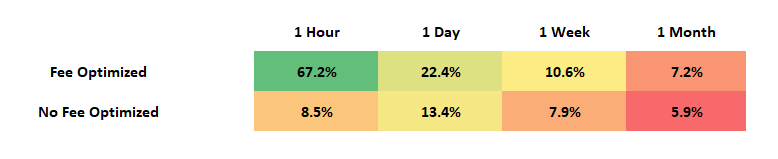
Figure 5: Each cell represents the comparison between a rebalancing strategy and HODL. A positive value means the strategy outperformed holding by that amount. Essentially, if the holding strategy performed +100% over the 1 year period, a positive percent means the rebalance strategy performed even better than +100%.
In figure 5 we see that all rebalancing strategies outperformed holding (based on the median portfolio performance). That means the median buy and hold strategy performs worse than the median of any rebalancing strategy.
Finally, we can compare the fee optimized rebalance results to the standard rebalance results so we can see the specific benefit that is generated from using fee optimization.

Figure 6: Each cell represents the benefit derived from fee optimization. Essentially, how much better does a portfolio perform when using fee optimization rather than no fee optimization.
As we previously discussed, we can see that the benefit of fee optimization grows as the rebalance frequency increases.
Conclusions
We can conclude from these results that rebalancing has tended to outperform a buy and hold strategy historically. In addition, we can see that the benefit of using a fee optimization strategy tends to increase with the frequency of the trading. The more frequently a strategy trades, the more benefit that is generated from the fee optimization.
Without fee optimization, the best performing strategy was a 1-day rebalance interval.

Threshold Rebalancing
To evaluate threshold rebalancing, we will examine 7 different threshold strategies. These will include a 1%, 5%, 10%, 15%, 20%, 25%, and 30% threshold rebalance. Similar to the periodic rebalancing portion of this study, we will compare the standard rebalance, fee optimized rebalance, and HODL results.
Each configuration will run 1,000 unique backtests for a total of 21,000 backtests.
HODL Results
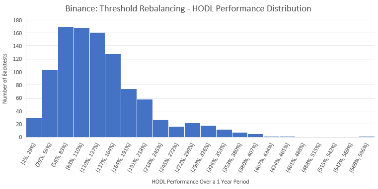
Figure 7: The above chart is an example of the portfolio performance distribution that we observed when no trading was done for the portfolio. 1,000 backtests were included in the histogram. After each backtest was run, it was placed into one of the performance buckets to create the curve you see. As an example, about 160 backtests produced performance results that ranged between 110% and 137% for the HODL strategy.
Over the 1-year period that was evaluated, portfolios that used a HODL strategy saw a median portfolio value increase of 115%. Notice that adjusting the rebalance threshold does not impact the median performance since a HODL strategy does not rebalance.
Small deviations in the HODL performance are observed in the results. These small deviations are simply the result of random chance. Based on the portfolio selections for the 1,000 backtests, we expect that the median performance will not be identical every time.
Regular Rebalance Results

Figure 8: The above chart is an example of the portfolio performance distribution that we observed when using a 15% threshold rebalancing strategy (with fee optimization). 1,000 backtests were included in the histogram. After each backtest was run, it was placed into one of the performance buckets to create the curve you see. As an example, about 98 backtests produced performance results that ranged between 173% and 197% for the 15% threshold rebalancing strategy.
Over the 1 year time period, regular threshold rebalances had a median performance ranging from 134.1% to 152.7%.
1% Threshold - 134.1% Median Performance
5% Threshold - 150.5% Median Performance
10% Threshold - 150.2% Median Performance
15% Threshold - 152.7% Median Performance
20% Threshold - 147.4% Median Performance
25% Threshold - 150.2% Median Performance
30% Threshold - 147.0% Median Performance
Fee Optimized Rebalance Results

Figure 9: The above chart is an example of the portfolio performance distribution that we observed when using a 1% threshold rebalancing trading strategy (with fee optimization). 1,000 backtests were included in the histogram. After each backtest was run, it was placed into one of the performance buckets to create the curve you see. As an example, about 118 backtests produced performance results that ranged between 152% and 189% for the 1% threshold rebalancing strategy.
Over the 1 year time period, fee optimized threshold rebalances had a median performance ranging from 156.5% to 258.3%.
1% Threshold - 258.3% Median Performance
5% Threshold - 197.2% Median Performance
10% Threshold - 179.1% Median Performance
15% Threshold - 172.1% Median Performance
20% Threshold - 163.2% Median Performance
25% Threshold - 164.1% Median Performance
30% Threshold - 156.3% Median Performance
Discussion
Combining the results, we can visualize the final performances as a grid.

Figure 10: Each cell in the grid represents the median performance of 1,000 backtests. The percentage represents the percent increase in value of the portfolio over the course of the 1 year period. Therefore, a 100% would represent the value of a portfolio doubling over the backtest period.
In figure 10 we can see that although the median portfolios leveraging a buy and hold strategy more than doubled in value over the course of a 1 year period, all threshold rebalancing strategies outperformed the HODL strategy.
This suggests that regardless of the selected threshold, rebalancing has historically tended to outperform holding.
When we narrow our evaluation to only comparing fee optimized rebalances with standard rebalances, we can see that fee optimization has a big impact on the results.

Figure 11: Each cell represents the median percent increase that each strategy has over buy and hold. Essentially, a positive value means the strategy outperformed buy and hold by that percent. Notice that if a portfolio using the HODL strategy increased in value by 100%, a positive value in this table would mean the rebalancing strategy performed even better (so greater than 100% in this example).
In figure 11 we see that the median rebalance strategy outperformed a simple HODL strategy in all cases that were studied. However, fee optimization was able to further build on performance increases to generate additional value.
Comparing only the two rebalancing strategies, we can see how much value was actually generated by the fee optimization algorithms used in the “fee optimized” rebalances.

Figure 12: Each cell represents the benefit derived from fee optimization. Essentially, how much better does a portfolio perform when using fee optimization rather than no fee optimization.
In figure 12 we can see the benefit of utilizing a fee optimized strategy. Keeping with the themes we saw in the periodic rebalancing case, we can see that fee optimization provides more benefit when there are frequent trades.
Conclusions
We see that similar to periodic rebalancing, threshold rebalancing has historically outperformed a simple buy and hold strategy. In addition, we see that the benefits of fee optimization grow as trading becomes more frequent.
Final Thoughts
After examining 33,000 backtests, we were able to consistently demonstrate the advantage of fee optimized rebalancing when compared to strategies that don’t use fee optimization. In addition, we were able to definitively produce results that suggest that portfolio rebalancing outperformed HODL strategies historically.
In fact, nearly 85% of all portfolios that were evaluated produced better results when using a rebalancing strategy when compared to HODL.
Additional Good Reads
How to Make a Crypto Trading Bot Using Python
A Comparison Of Rebalancing Strategies for Cryptocurrency Portfolios
Common Rebalance Scenarios in Crypto
Threshold Rebalancing for Crypto Portfolio Management
What Is DeFi? Guide to Decentralized Finance
About Us
Shrimpy is an account aggregating platform for cryptocurrency. It is designed for both professional and novice traders to come and learn about the growing crypto industry. Trade with ease, track your performance, and analyze the market. Shrimpy is the trusted platform for trading over $13B in digital assets.
Follow us on Twitter for updates!